Intro to Quantum Mechanics

Hello hello! I’m a first-year at Wellesley College, an all-women’s liberal arts college in Massachusetts. I’m teaching a series of crash courses on Chemistry – you can find the page here. Without further ado, let’s dive into the world of quantum mechanics – no previous experience necessary, but it gets intense, so follow along!

(Bear in mind that you do not need to understand everything in this tutorial.)

---

What is a wave?

Think of ripples in a pool, or sound produced by the radio. Waves are periodic disturbances/oscillations that pass through a medium (i.e. air, water, etc.).

A cycle is the repeating unit of a wave. Multiple cycles make up a continuous wave.

The main equation we use to measure waves is v = λf. Think about it, it’s just the velocity equation “v = d/t” in disguise. The velocity of a wave is v. The symbol λ is the wavelength, which is just a distance (d). And f is the frequency is the amount of time it takes for a cycle to travel the distance of that wavelength, so it’s just time (t).

Of course, we can substitute the speed of light constant, c = 3×10⁸ ms^-2 into the equation above so that we can calculate the wavelength or frequency of an electromagnetic wave, which travels specifically at that velocity in a vacuum. This allows us to transition nicely into our next section.

Electromagnetic Waves

What exactly is electromagnetic radiation? If we break apart the word, we see “electric” and “magnetic”. We see two perpendicular fields – an electric field and a magnetic field – that propagate one another.

Of course, what we really can see of electromagnetic radiation, is visible light. That’s only a tiny portion of the spectrum though, other examples of EM radiation include ultraviolet light, infrared rays, X-rays, and radio waves, and they all have different applications in our lives.

Spectroscopy

Spectroscopy is a way of studying absorptions and emissions of electromagnetic radiation by matter. All kinds of spectra result from transitions between the ground state and the excited state.

As you may know, electrons exist in different orbitals around the atom. Some of these orbitals are at a lower energy state. When an electron moves from an orbital of a higher energy to one of lower energy level, it will emit a packet of energy called a photon. When an electron jumps to a higher energy level, it absorbs a photon.

Essentially what these diagrams represent are the wavelengths of the photons absorbed and emitted for a specific element, since the transitions are “quantized” and only occur for specific wavelengths. This serves as a sort of “bar code” to allow scientists to identify what elements are in a sample.

Quantum Theory of Radiation

The Dual Nature of Radiation

Light was previously known to exhibit wave properties, such as interference and diffraction. However, a century or so ago, it was observed that light could also behave as a particle (i.e. a photon).

The energy carried by these photons is proportional to the frequency of the light: E = hf, where h is Planck’s constant: h = 6.6261×10^-34 J^-1.

We have to accept the wave-particle duality of electromagnetic radiation!

Photoelectric Effect

The process by which electrons are ejected from a metal surface when light strikes the surface is called the photoelectric effect. The kinetic energy of the ejected electron is observed to be independent of the intensity of radiation, and the photoelectric effect is completely absent below a certain threshold frequency. These phenomena couldn’t be explained by classical physics, and Einstein won a Nobel Prize for his explanation:

0.5mv² = hf – φ

The left side is the electron’s kinetic energy, which is greater than or equal to 0.

hf is the energy of the photon (E = hf), and φ is the work function – the minimum energy required to remove an electron from the surface (specific to the metal in question).

At the threshold frequency the kinetic energy of the electrons is 0. Below that, no electrons are ejected. The threshold frequency can be given by this equation:

hf = φ

Matter Waves: Dual Nature of Matter

Louis de Broglie proposed if light has wave-particle duality, then matter, which is supposedly a particle, may also have wave-like properties.

Given the definition of momentum (p = mv), a particle with mass m and speed v should have a wavelength:

λ = h/p = h/mv

Quantum effects are unobservable for macroscopic objects (technically, you have a de Broglie wavelength!), but for a microscopic object, we obtain a wavelength of atomic dimensions. Electrons show interference patterns characteristic of waves (i.e. diffraction).

Heisenberg’s Uncertainty Principle

According to Heisenberg’s uncertainty principle, it is impossible to make simultaneous and exact measurements of both the position (x) and momentum (p) of a particle.

(Δx)(Δp) ≈ h

So, if Δx is small, then Δp will be large, and vice versa. The more precisely the position is known, the greater the uncertainty in momentum. The uncertainty is inherent and cannot be reduced by improvement in measurement technique.

Since it’s not possible to specify the trajectory of microscopic particles such as electrons, the Bohr model of the atom (the one you learned in school, with the orbits of electrons around the nucleus) is incompatible with this understanding.

Wave Mechanics and Schrödinger’s Equation

If you’re confused at this point, don’t worry! Richard Feynman himself once said, “I don’t understand it. Nobody does.” You’re normal.

Each state of a particle is associated with a wavefunction. Given the wavefunction corresponding to a particular state, one can calculate the probability of finding the particle in any specified region of space.

To get the wavefunction, we need to solve Schrödinger’s equation. This is the central equation of quantum mechanics.

HΨ = EΨ

H is the Hamiltonian operator, Ψ is the wavefunction and E is the energy. That’s all you need to know for now.

(Solving the equation is super, super, super complicated. So let’s just go ahead and discuss the solutions to the Schrödinger equation.)

Solving the equation (let’s say we did) yields a series of wavefunctions and energies. (Actually, the hydrogen atom can be exactly solved. All the other elements have approximate solutions.)

1. The wavefunction (orbital) gives information about the position of an electron.
2. The quantized energy levels are useful in understanding line spectra.

Four Quantum Numbers

There are four quantum numbers needed to specify the state of an electron in an atom, which we will discuss next.

1. Principal Quantum Number
   Symbol: n
   Permitted values: 1,2,3,4…any positive integral value starting with 1
   n determines the size of an orbital and the distance of the electron from the nucleus. n=1 corresponds to the orbital closest to the nucleus, and is the lowest energy orbital.
   The energy for an electron is given by ; where k for H is 2.179×10^-18 J.
   Because of the n^2 in the denominator, the spacing between successive orbitals decreases with increasing n.
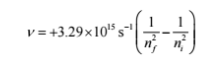
   An electron falling from a higher n level will emit a photon, which will have the same energy as the energy difference between the electron’s initial and final states. This can be represented by the Bohr-Einstein relationship:
   To get the frequency of the emitted light, we can use the Rydberg formula:
   
2. Orbital Angular-Momentum Quantum Number
   Symbol: l
   Permitted values: 0,1,2…n-1
   The quantum number l determines the shape of the orbital. The letter symbols for l are used for orbital designation so that s (l=0), p (l=1), d (l=2), f (l=3), and g (l=4). For example, the s orbitals are all spherical in shape while the p orbital has a dumbbell shape.
3. Magnetic Quantum Number
   Symbol: m_l
   Permitted values: –l, –l+1, –l+2…0,…l-2, l-1, l; all integral values between -l and +l including 0
   The magnetic quantum number determines the orientation of the orbital and the behavior of electrons in a magnetic field. For example, there are 3 degenerate 2p atomic orbitals that split into three different energy levels, which correspond to the three different values of the magnetic quantum numbers for l=1.
4. Spin Quantum Number
   Symbol: ms
   Permitted values: -1/2, +1/2
   In the Stern-Gerlach experiment, it was shown that a beam of atoms would be split in a magnetic field. The direction in which the electrons move is based on the spin of an electron, and can’t really be explained via classical mechanics.

Physical Meaning of Wavefunctions

Orbitals are regions in which electrons are the most likely to be found. The wavefunction Ψ is a set of numbers, in which one particular value is assigned to every point in space.

Let’s look at an example. The wavefunctions for H are the s, p, d, and f orbitals, and the 1s orbital is an exponential decay function (no need for memorization, just observe):

where a0 is a constant called the Bohr radius and r is the distance of the electron from the nucleus.

The 1s wavefunction only depends on r, but with other wavefunctions the variables can also depend on θ (latitude) and φ (longitude). We express the wavefunction in spherical polar coordinates instead of Cartesian, so we can go out from the nucleus a distance r to a specific θ and φ on the sphere to compute the value of ψ at that point (a plain number with a sign).

Another example with the hydrogen atom is the 2px orbital (don’t sweat it!):

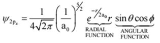
We can separate this wavefunction into two components – the radial function depends on r, while the angular function depends on θ and φ.

The general expression for the hydrogen atom wavefunction is as follows:

and depends on the three quantum numbers (n, l, m_l), and three coordinates (r,θ,φ). The hydrogen atom has an infinite number of orbitals even though only the lowest energy 1s orbital is occupied in the ground state of the atom.

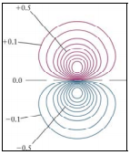
Born’s Interpretation of Orbitals

So we know now that Bohr’s model doesn’t really work with what we know. Schrödinger describes electrons through orbitals in his mechanical model. Max Born further sought symmetry between light and matter when trying to interpret the wavefunction.

Born proposed that the probability of finding an electron at a point is equal to the square of the wavefunction at that point – the quantity ψ² is called the probability density/electron density.

For example, if we look on the red graph below, we see that the probability of finding that electron decreases as the distance from the nucleus increases after a certain point.

Image Source: TWDK

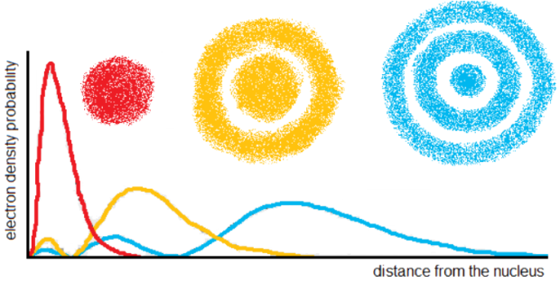
Nodes

A node is a surface on which the electron density is 0. They can be classified as either radial or angular. Where can you identify nodes on the diagram above?

Radial nodes occur at a fixed radius and are spherical in shape. The number of radial nodes is (n–l-1). For example, the 4s atomic orbital contains 4-0-1=3 radial nodes.

Any node that isn’t spherical is angular. The number of angular nodes is l. Nodal planes and nodal cones are most common.

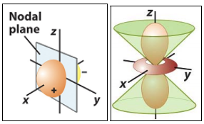
Image Source: Professor Chris A

For your further information: The total number of nodes is n-1. The sign of the wavefunction switches when one crosses a node (the sign does NOT correspond to electrical charge).

Graphical Representations of Orbitals

Pretty pictures! There are seven (!!!) methods for graphically representing the atomic orbitals of H. This is our last section, we’re almost done!

1. Radial functions (R(r)) and Radial functions squared (R^2(r))
   
2. Radial distribution function (RDF)
   We ask, “What is the probability of finding the electron at a certain distance r from the nucleus, irrespective of angle?” So, we multiply the probability density by the volume of the associated spherical shell:
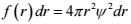   f(r) is the radial distribution function.
   The maxima correspond to radii at which the electron is most likely to be found, while the minima correspond to radial nodes.
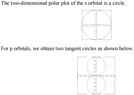
   We can see that the most probable distance of the H atom electrons increases with increasing principal quantum number, which explains why an s electron has a great chance of being closer to the nucleus than a p electron, which is in turn more likely to be near the nucleus than a d electron.
3. Two Dimensional Polar Plots (Represents only the θ part)
   The above representations don’t show how the probability depends on the angular coordinates, which specify the position of a point in space.
   
4. Three Dimensional Polar Plots (Represents both the θ part and the Φ part)
   These polar plots will not show spherical nodes.
   The 3-D polar plot for an s orbital is a sphere.
   The three p orbitals (l=1) corresponding to the three m_l values point in the x, y, and z directions.
   There are five d orbitals (l=2) corresponding to the five m_l values.
   
5. Probability Density Plots
   We can represent the value of Ψ² by the density of dots in a picture:
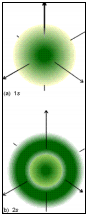   which provide radial and angular information. (Almost there! Hold on…)
6. Two-Dimensional Contour Maps
   Similar to topographical maps of geographical regions, these maps show contours of constant electron density.
   
7. Three-Dimensional Contour Surfaces of Constant Probability
   Typically, this is what you’re used to seeing in high school textbooks when looking at representations of atomic orbitals. It’s my personal favorite because it makes sense – we draw surfaces in space on which the value of Ψ² is constant. These three-dimensional surfaces of constant probability are also known as isoelectron density surfaces.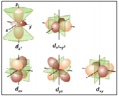
   

   The 3d orbital

   

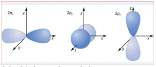
   The 2p orbital

    

Want to play around with these orbitals some more? Click here to find the program “Orbital Viewer”.

---

Congratulations for making it to the end of my post! You’re great (I know this was information at a more challenging level than casual, easy reading).

If I still leave any questions unanswered, please leave it in the comment section below and I will try my best to address them.

Keep checking back for more! (Or better yet, subscribe to my blog!)

Lots of love,